
TL;DR: Using a layer-by-layer logit-lens hook, I probed the hidden state representations of fine-tuned InternVL3-2B and 8B models across 28 layers. The 2B model settles on the final answer earlier than the 8B model. Most early and middle layers are noisy, with the correct answer emerging mainly in the final third of the network.
In multimodal vision-language models (VLMs), detecting hallucination-identifying objects, attributes, counts, relationships mentioned in text that do not actually exist in an image—requires tightly bound visual grounding and text alignment.
When a fine-tuned VLM like InternVL3 outputs a hallucination flag, at what depth (layer) does this decision form? Does a larger model settle on its output earlier?
To check this, a probing was performed using logit-lens across two model variants: InternVL3-2B and InternVL3-8B.
Experimental Setup
Task & Dataset Format
The models were evaluated on 1232 samples of our IITH LID-test dataset (structured accordingly for MS-Swift fine-tuning). The models receive an image and a candidate caption, and are instructed to output either:
"None"if no hallucination exists.- A comma-separated list of hallucinated words/phrases if inconsistencies exist.
An instance of the test structured file looks like this:
[
    {
        "messages": [
            {
                "role": "system",
                "content": "You are InternVL3, a multimodal model that reads images and text. Your task is to detect hallucinated words in image descriptions. Hallucinations are objects, counts, positions, attributes, relationships, or actions/details not present in the image. Ignore subjective interpretations.\n\nInput: an image and a candidate description.\nOutput format: \n- \"None\" if the description fully matches the image.\n- Otherwise, a comma-separated list of hallucinated words/phrases. \nDo not add any extra commentary. Be conservative - only flag clear visual inconsistencies.\n"
            },
            {
                "role": "user",
                "content": "Image: <image> Description: The image features a large construction site with a building under construction. The building is surrounded by scaffolding, and there are several construction workers on the site. The workers are scattered throughout the scene, with some closer to the building and others further away.\n\nIn addition to the workers, there are two trucks visible in the scene, one near the left side of the image and the other towards the right side. The presence of these vehicles suggests that they may be involved in the construction process or transporting materials to the site.\n\nFind hallucinated words from the description that don't match the image."
            },
            {
                "role": "assistant",
                "content": "two trucks"
            }
        ],
        "images": [
            "/path/to/image.jpg"
        ]
    }, ...
]
How probing works
LayerProbe registers a forward hook on every decoder layer
(model.language_model.model.layers). During model.chat(...), each hook
grabs the hidden state at the last token position (hidden[:, -1:, :]) after that layer runs. Because generation is autoregressive, one new token’s hidden state is captured per layer per generation step. Concatenating these across steps reconstructs a per-layer “what would this layer have output” sequence for the whole generated response.
After generation, decode_per_layer passes each layer’s collected hidden states through the model’s final norm and lm_head, argmaxes the logits and decodes the resulting token ids. This gives one decoded string per layer, per example — the layer’s “guess” at the final output if you stopped the network there.
This is a logit-lens on the generation trajectory (one hidden vector per step, taken with KV-cache), not a single-pass probe over a full prefill sequence.
The core of it, straight from probe_layers.py:
class LayerProbe:
    def __init__(self, language_model):
        self.lm = language_model
        self.layers = self.lm.model.layers
        self.norm = self.lm.model.norm
        self.lm_head = self.lm.lm_head
        self.handles = []
        self.trace = {i: [] for i in range(len(self.layers))}

    def _make_hook(self, idx):
        def hook(module, inputs, output):
            hidden = output[0] if isinstance(output, tuple) else output
            self.trace[idx].append(hidden[:, -1:, :].detach())
        return hook

    def __enter__(self):
        for i, layer in enumerate(self.layers):
            self.handles.append(layer.register_forward_hook(self._make_hook(i)))
        return self

    def __exit__(self, *args):
        for h in self.handles:
            h.remove()

    def decode_per_layer(self, tokenizer):
        results = {}
        for idx, hiddens in self.trace.items():
            if not hiddens:
                continue
            seq = torch.cat(hiddens, dim=1)  # (1, num_gen_steps, hidden)
            with torch.no_grad():
                logits = self.lm_head(self.norm(seq))
            token_ids = logits.argmax(dim=-1)[0].tolist()
            results[f"layer_{idx}"] = tokenizer.decode(token_ids, skip_special_tokens=True)
        return results
Used as a context manager around model.chat(...), so hooks are attached
only for the duration of one generation and removed right after:
with LayerProbe(model.language_model) as probe:
    with torch.no_grad():
        response = model.chat(
            tokenizer, pixel_values, question, gen_config, history=None, return_history=False,
        )
    layer_outputs = probe.decode_per_layer(tokenizer)
Running it
After fine-tuning on the LID train data, we use the best trained checkpoint for probing.
CUDA_VISIBLE_DEVICES=2 python path/to/probe_layers.py \
    --val_dataset /path/to/test_structured_internvl3.json \
    --model_path path/to/sft_checkpoints/internvl3_2b/best-ckpt-merged \
    --output layer_probe_2b.jsonl \
    --max_new_tokens 32
The probe file runs inference and dumps per-layer decoded predictions to JSONL, a row may look like this:
{
  "index": 0,
  "image": "path/to/image.jpg",
  "ground_truth": "two trucks",
  "final_generation": "trucks",
  "layer_predictions": {"layer_0": "...", "layer_1": "...", ..., "layer_27": "..."}
}
Analysis
Note: The codes for the plots and the analysis on the jsonl files were generated using Gemini.
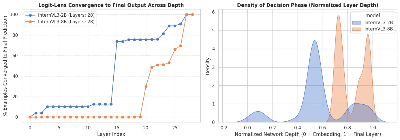
Left — convergence to final output 2B sits around 10–13% match through layers 0–14, then jumps to ~74% at layer 15 and gradually to 100% by layer 27. 8B stays at 0% match through layer 19, jumps to ~30% at layer 20, and 60s% by layer 26 before reaching 100% at layers 27–28.
Right — KDE 2B has a small early bump near 0.1 depth plus a dominant peak around 0.55 normalized depth. 8B’s distribution is concentrated later, with peaks around 0.72–0.75 and 0.9–0.95 depth — consistent with the later jump seen in the convergence curve.
Layer-to-layer stability heatmaps
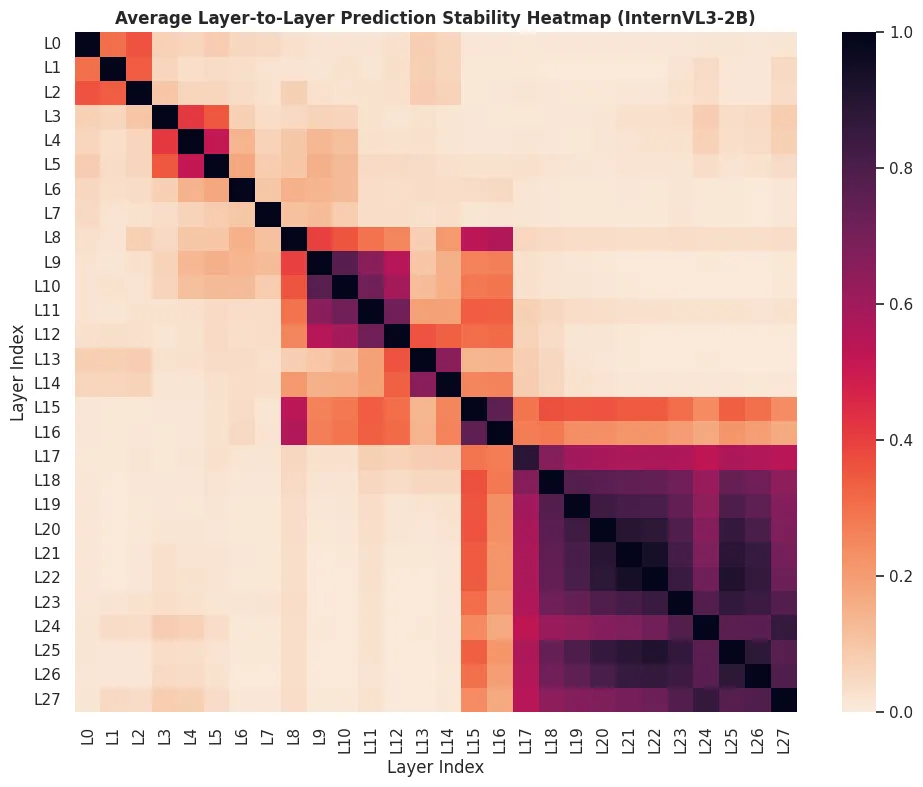
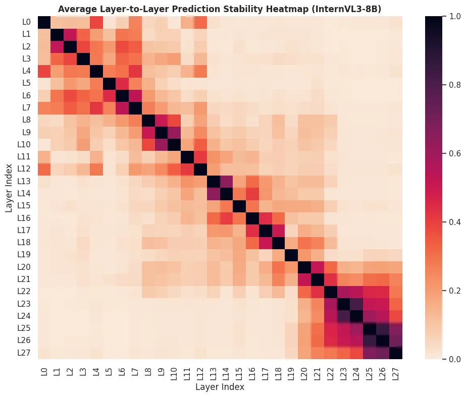
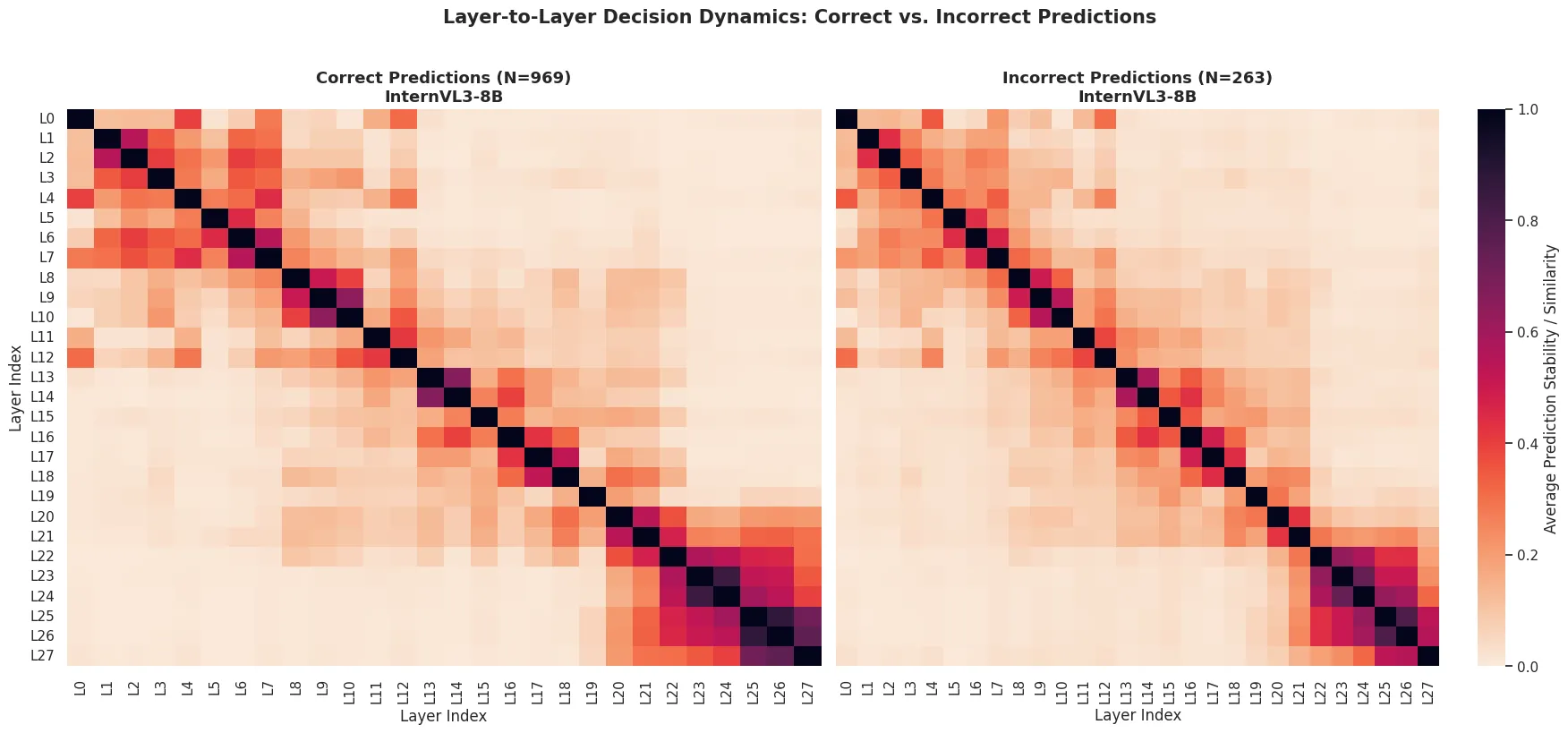
Predictions are similar across nearby layers, especially in small groups like L3–L5 and L8–L12. In the later part of the network, predictions become highly similar across many layers (about L17–L27 in the 2B model and L20–L27 in the 8B model), once the predictions get close to the final answer.
Correct vs. incorrect predictions
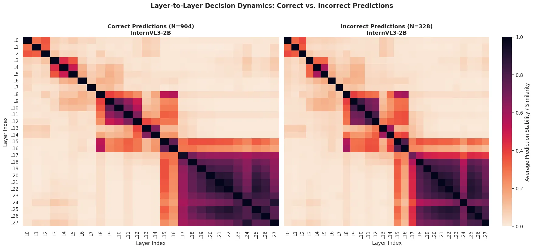
| Model | Correct | Incorrect | Total |
|---|---|---|---|
| InternVL3-2B | 904 | 328 | 1,232 |
| InternVL3-8B | 969 | 263 | 1,232 |
The two heatmaps within each pair look qualitatively similar. Whatever drives the incorrect answers isn’t showing up as a distinct layer-agreement pattern here.
An example
Example 0, InternVL3-2B. Ground truth: two trucks. Final output: trucks.
| Layer | Decoded output |
|---|---|
| layer_0 | wh multiplicマン |
| layer_1 | with�loads |
| layer_2 | � car |
| layer_3 | sTac trucks |
| layer_4 | s especially trucks |
| layer_5 | ss trucks |
| layer_6 | s limbloads |
| layer_7 | Group� vehicles |
| layer_8 | Aline car |
| layer_9 | s�-mounted |
| layer_10 | s谢邀loads |
| layer_11 | 谢邀manship |
| layer_12 | 谢邀manship |
| layer_13 | 谢邀manship |
| layer_14 | 0谢邀 gim |
| layer_15 | None谢邀manship |
| layer_16 | 沓manship |
| layer_17 | 觋olver |
| layer_18 | None院副院长 are |
| layer_19 | None委宣传auce |
| layer_20 | None诓, |
| layer_21 | Noneucks, |
| layer_22 | Noneucks |
| layer_23 | truckiggers, |
| layer_24 | truck trucks |
| layer_25 | Noneucks |
| layer_26 | trucks, |
| layer_27 | trucks |
The early layers produce unrelated tokens. Some middle layers repeatedly produce unrelated text. The output only starts looking like “trucks” around layer 23 and becomes stable by layers 26–27.